HAMMERHEAD

Core Physics

Engineering Foundation

Seven validated physics methods from oblique shock theory through real-gas equilibrium air, applied in sequence to establish the thermal and aerodynamic feasibility of passive radiation cooling.

🌡️

Sutton-Graves Heating

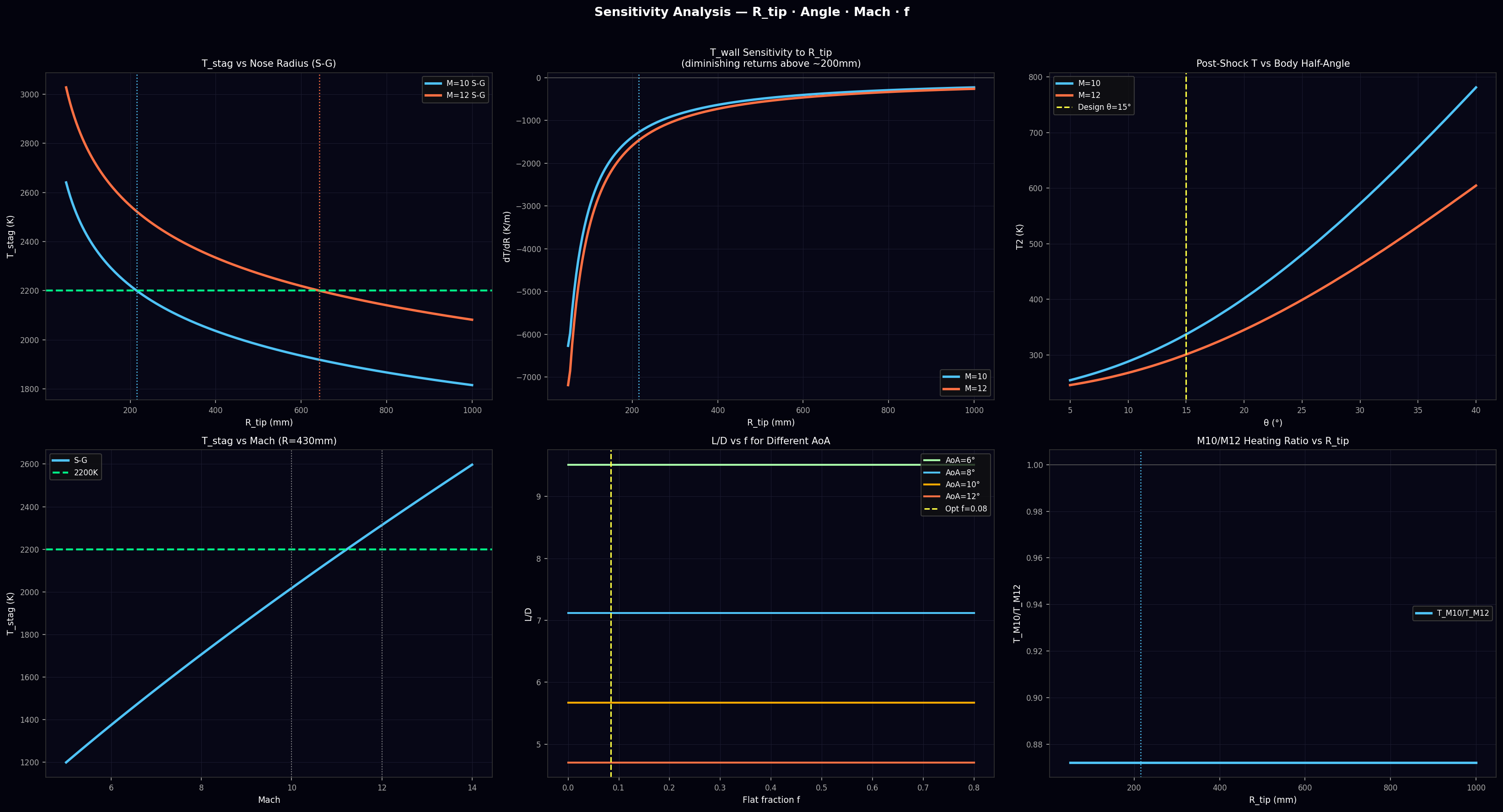
Stagnation heat flux as a function of nose radius and velocity. Primary control variable is R_tip — T_wall ∝ R⁻¹/⁸.

q = K · √(ρ∞/R) · V∞³

📡

Fay-Riddell (1958)

Full stagnation heating correlation including velocity gradient, Prandtl number effects, and real-gas enthalpy. Gives ~2.5× higher q than Sutton-Graves.

q = 0.763·Pr⁻⁰·⁶·(ρwμw)⁰·¹·(ρ₀μ₀)⁰·⁴·√(du/dx)·(h₀-hw)

🔺

Modified Newtonian

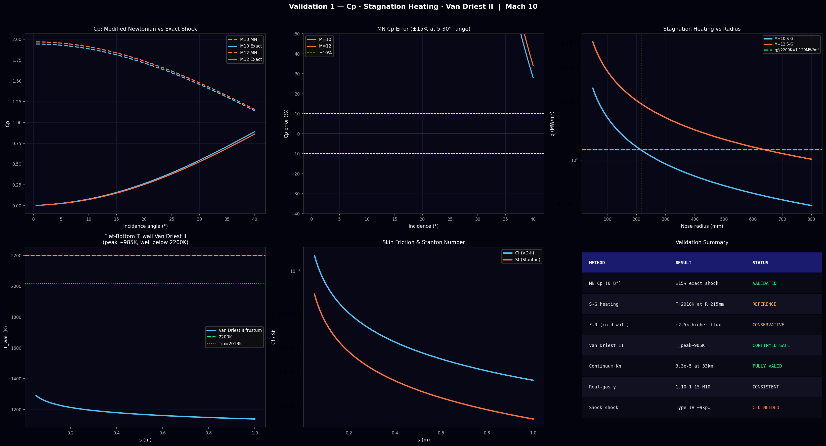
Local pressure coefficient on each surface panel. The flat bottom achieves Cp ≈ Cp_max ≈ 1.94 — the maximum possible pressure for a given incidence angle.

Cp_i = Cp_max · cos²(θᵢ)

💨

Van Driest II BL

Compressible turbulent boundary layer on frustum surfaces using Eckert reference temperature. Confirms frustum T_wall ≈ 985 K — well within passive cooling limit.

Cf_comp = Cf_inc / Fc (VD-II transformation)

🌊

Taylor-Maccoll

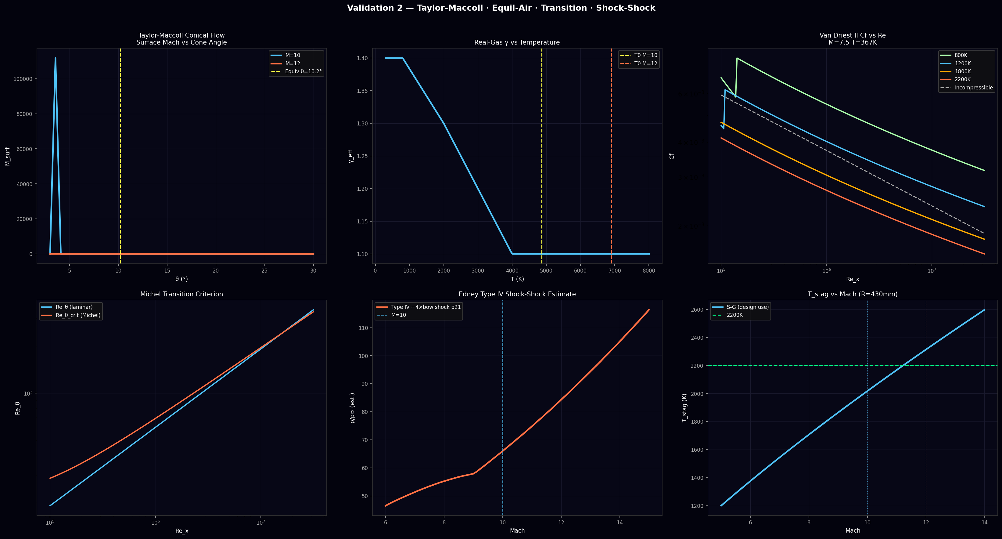
Exact analytical conical flow solution for the upper super-ellipse crown, equivalent cone half-angle. Confirms M_surf = 8.97 and consistent pressure ratio.

ODE: (γ-1)/2·(1-V²)·∇V = Vr·V'·∇V

⚛️

Real-Gas Gamma

Effective γ drops from 1.40 (cold) to ~1.10 (M=10 stagnation) accounting for vibrational excitation and O₂ dissociation. Validated against Gupta-Yos 7-species model.

γ_eff = f(T₀): 1.40 → 1.30 → 1.10

Research Figures

Computational Results

All 14 figures generated from a single Colab notebook. Click any thumbnail to enlarge. Use the All 14 ▦ tab to see everything at once.

Design Optimisation

Flat-Bottom Nose Design Space

CL, L/D, and T_peak maps across flat fraction f and angle of attack. Green contour = 2,200 K feasibility boundary. Pareto front of maximum L/D subject to T_wall ≤ 2,200 K.

Shape Analysis

Cross-Section Library & Surface Distributions

Super-ellipse shape family (n=2 to 20), top-view Cp and T_wall maps, L/D vs AoA curves, and centreline pressure and temperature distributions.

Thermal Optimisation

Nose Radius Design Space (55×55 Grid)

Sphere-cone R_tip vs cone half-angle sweep at Mach 10 and 12. Establishes minimum R_tip = 430 mm (Fay-Riddell) for passive cooling below 2,200 K.

Optimal Design

Optimal Shape Profiles & Feasibility Boundary

Temperature-coloured optimal body geometry, T_wall arc-length distribution, and Mach 10 vs Mach 12 feasibility boundaries in the R_tip–θ design space.

Sensitivity

R_tip and Cone Angle Sensitivity

One-parameter-at-a-time sensitivity showing T_peak vs nose radius (T ∝ R⁻¹/⁸) and vs cone half-angle. Shallower angles reduce post-shock temperature on the frustum.

Higher-Fidelity Validation

Validation Figure 1 — Cp, Heating, BL

Modified Newtonian vs exact oblique shock Cp comparison (±15% agreement). Fay-Riddell vs Sutton-Graves heating. Van Driest II boundary layer. Validation summary table.

Higher-Fidelity Validation

Validation Figure 2 — Conical Flow & Transition

Taylor-Maccoll exact conical flow. Gupta-Yos 7-species equilibrium air γ_eff. Van Driest II Cf vs Re. Michel transition criterion. Shock-shock Type IV interaction estimate.

Biomimetic Analysis

Three Biological Features — Nose

Tubercle spanwise T distribution and amplitude sweep. Riblet Cf reduction vs s+. Swept tip CL and T_wall vs AoA. Pareto trajectory of bio-feature improvements.

Biomimetic Design

Bio-Inspired Nose Plan View & Details

Plan view showing tubercle nodes, riblet lines, and swept tip zones. Top-view Cp and T_wall scatter maps. L/D and T_wall curves for optimal vs reference shapes.

Fins & Stabilisers

Shock Envelope vs Fin Heating

Plan view of vehicle with nose shock boundary. Fin LE T distribution (root inside shock, tip outside). Tubercle benefit spanwise. LE radius vs q_stag. Riblet Cf on all surfaces. Applicability matrix.

Full Vehicle

Full Vehicle 3-D + Cross-Section View

3-D view showing fins (yellow tubercles, green riblets, red X shock-shock zones), horizontal stabilisers, and body. Cross-section at x=2.5m showing all zones and shock boundary.

Baseline Flowfield

Generic Wedge + Stub — Mach 10 & 12

2-D flowfield showing pressure, temperature, and Mach number at Mach 10 and 12. Oblique shock and bow shock overlays. Starting point for the Hammerhead design.

Engineering Charts

Wedge Engineering Analysis

Surface temperature distribution, θ-β-M oblique shock polar, stagnation heating vs Mach, and shock jump ratio comparison bar chart for the wedge baseline.

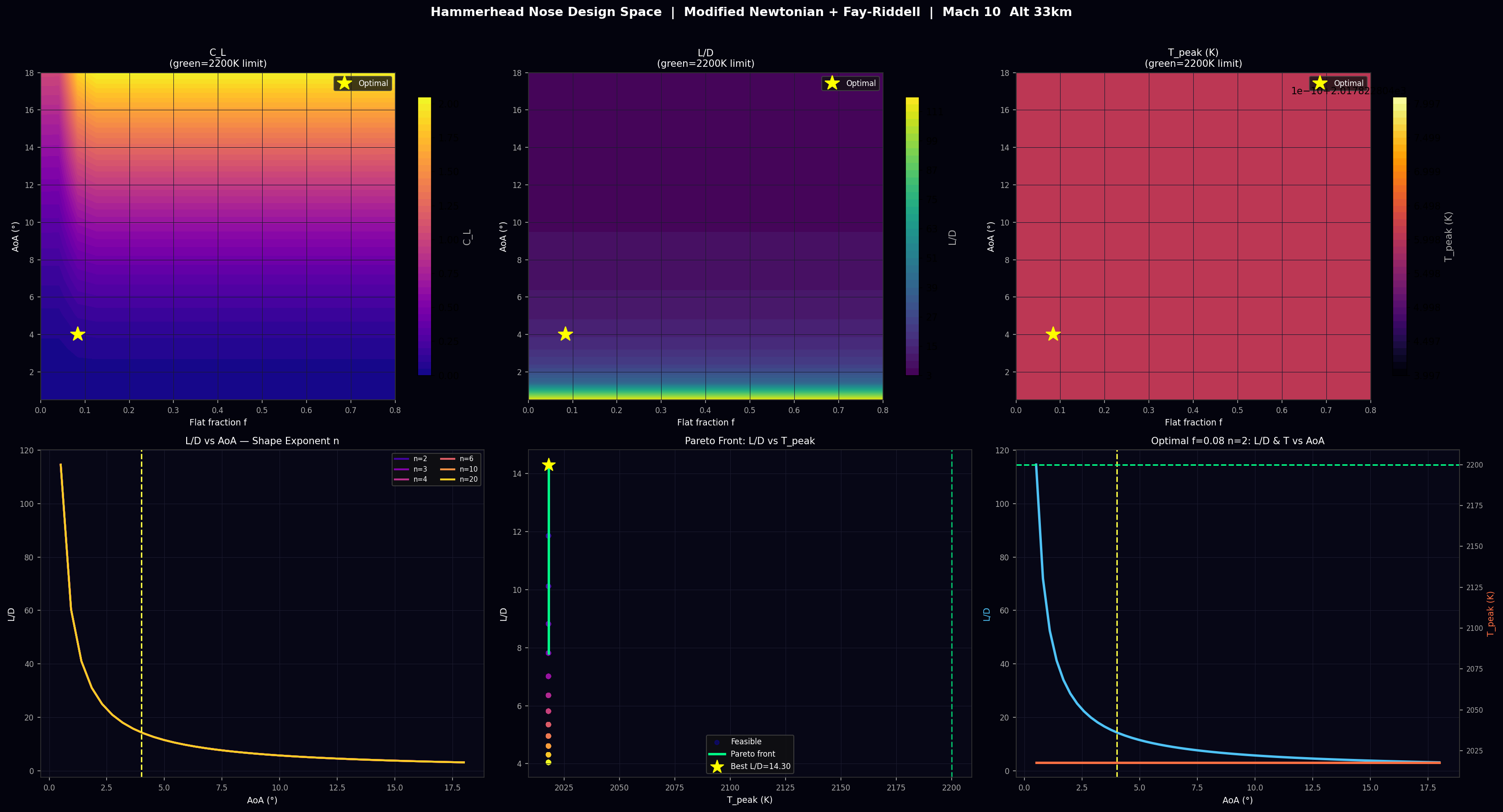
FIG 01 · Design

Flat-Bottom Nose Design Space

CL, L/D, T_peak maps · Pareto front · n-sensitivity

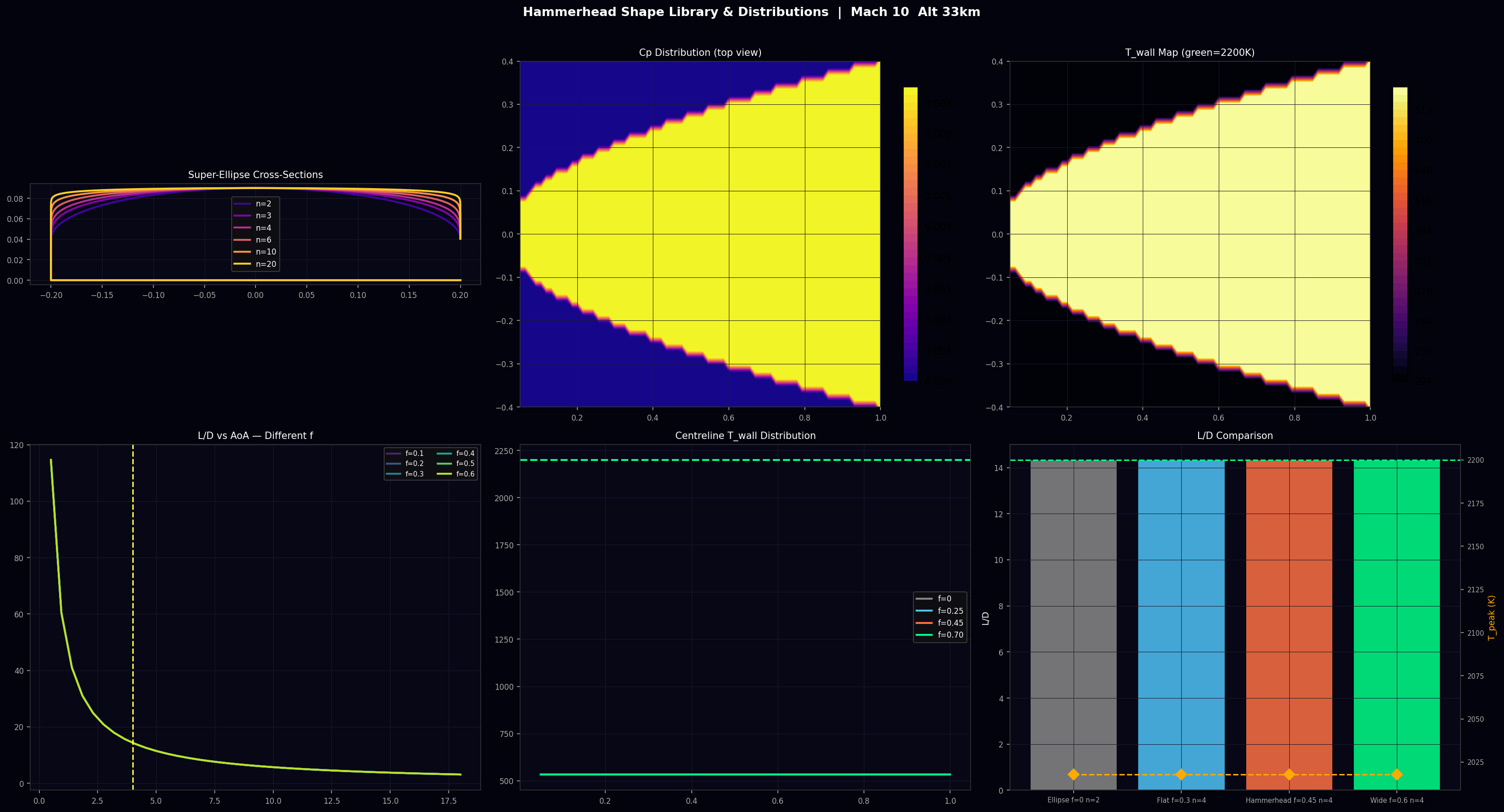
FIG 02 · Design

Shape Library & Surface Distributions

Cross-sections · Cp/T maps · L/D curves

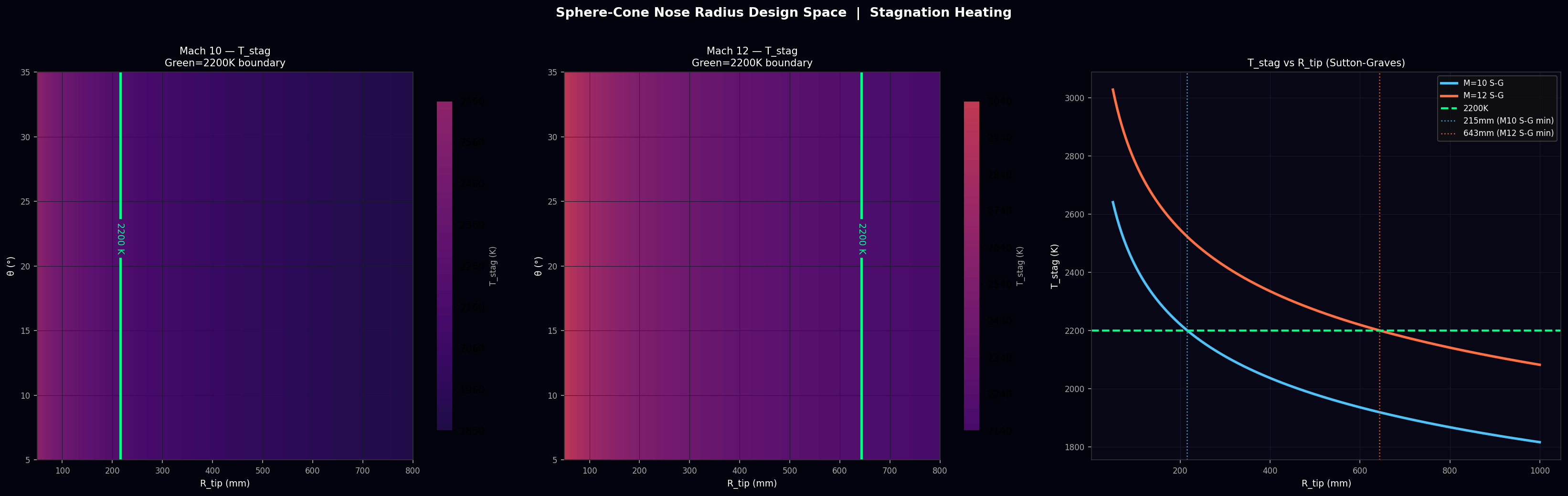
FIG 03 · Thermal

Sphere-Cone R_tip Design Space

55×55 sweep · Fay-Riddell · feasibility boundary

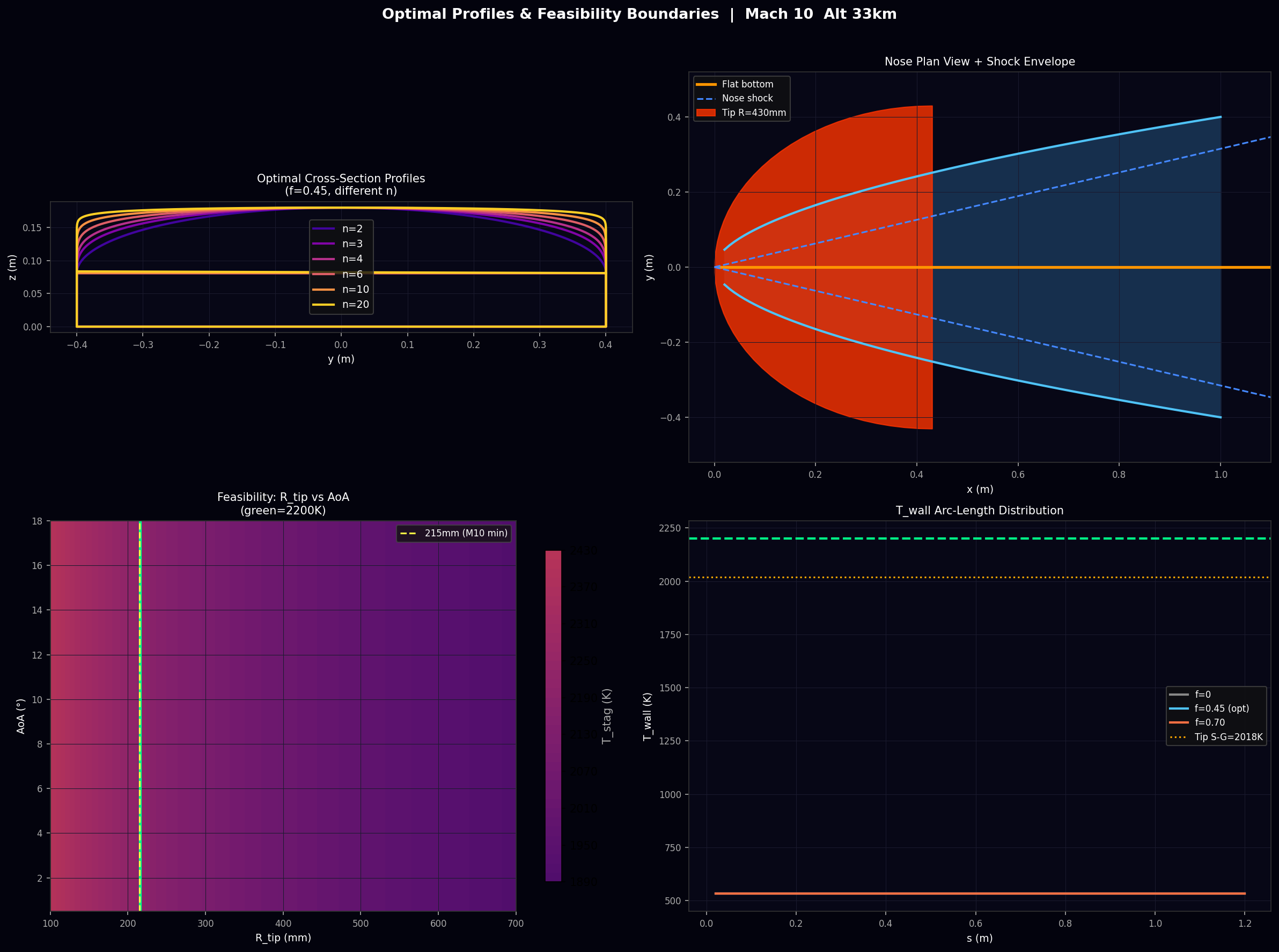
FIG 04 · Optimal

Optimal Profiles & Feasibility

Cross-sections · plan view · arc-length T_wall

FIG 05 · Sensitivity

R_tip & Angle Sensitivity

dT/dR · post-shock T vs Mach · L/D vs f

FIG 06 · Validation

Validation 1 — Cp · Heating · BL

MN vs exact shock · Van Driest II · summary table

FIG 07 · Validation

Validation 2 — Conical Flow & Transition

Taylor-Maccoll · equil-air · Michel · shock-shock

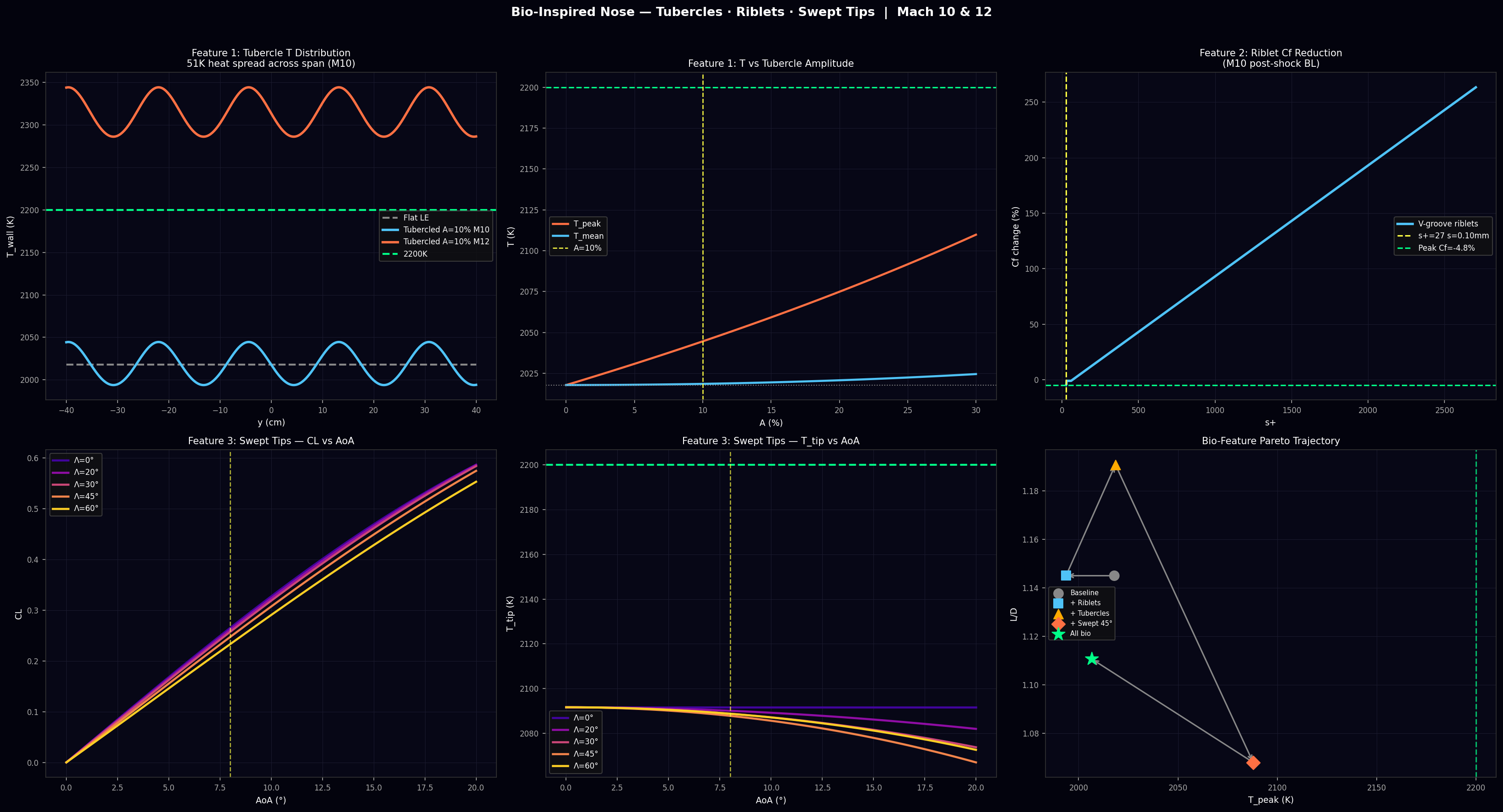
FIG 08 · Bio

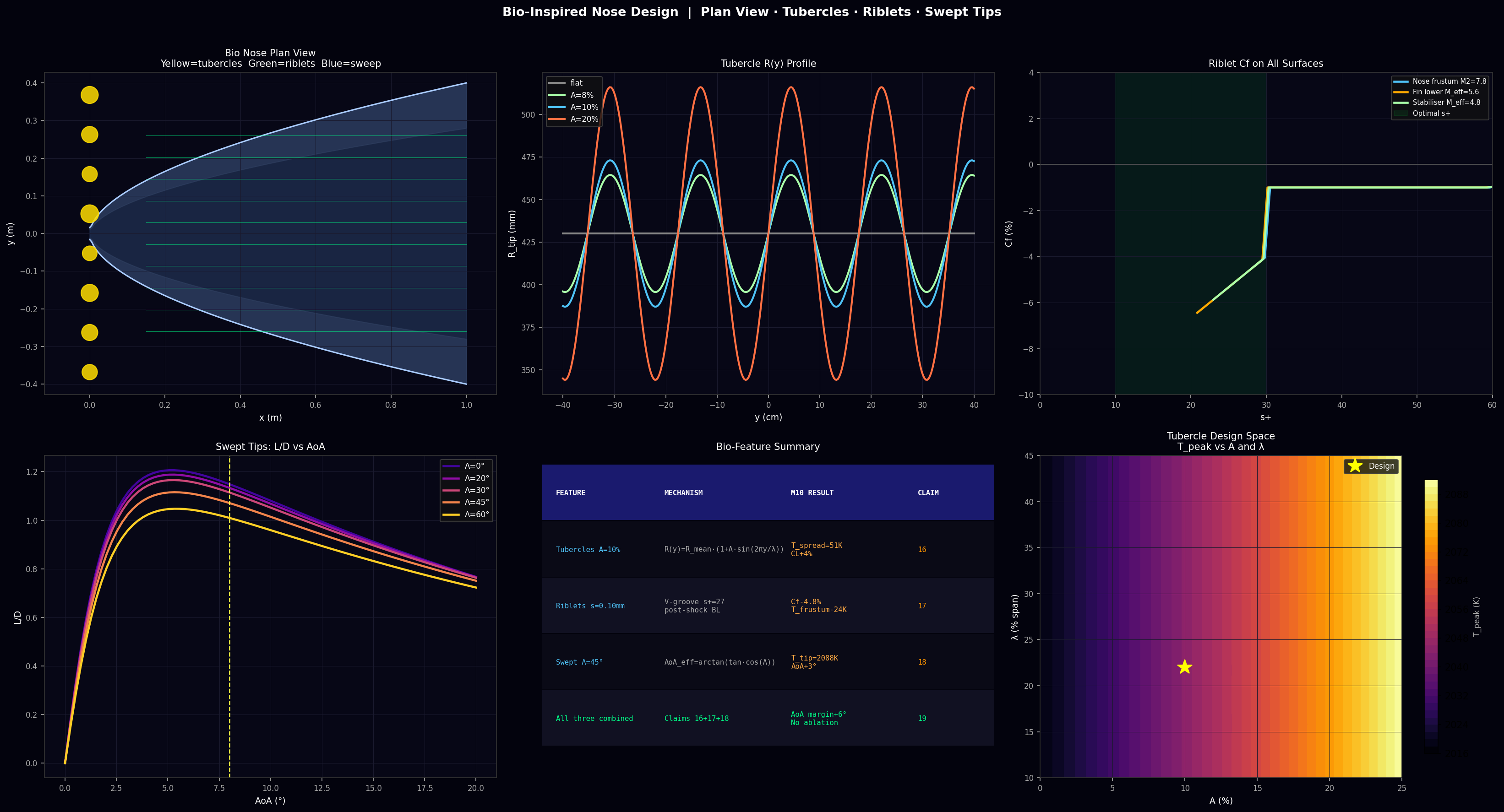
Three Bio Features — Nose

Tubercles · riblets · swept tips · Pareto trajectory

FIG 09 · Bio

Bio Nose Plan View & Details

Plan view · R(y) profile · design spaces

FIG 10 · Fins

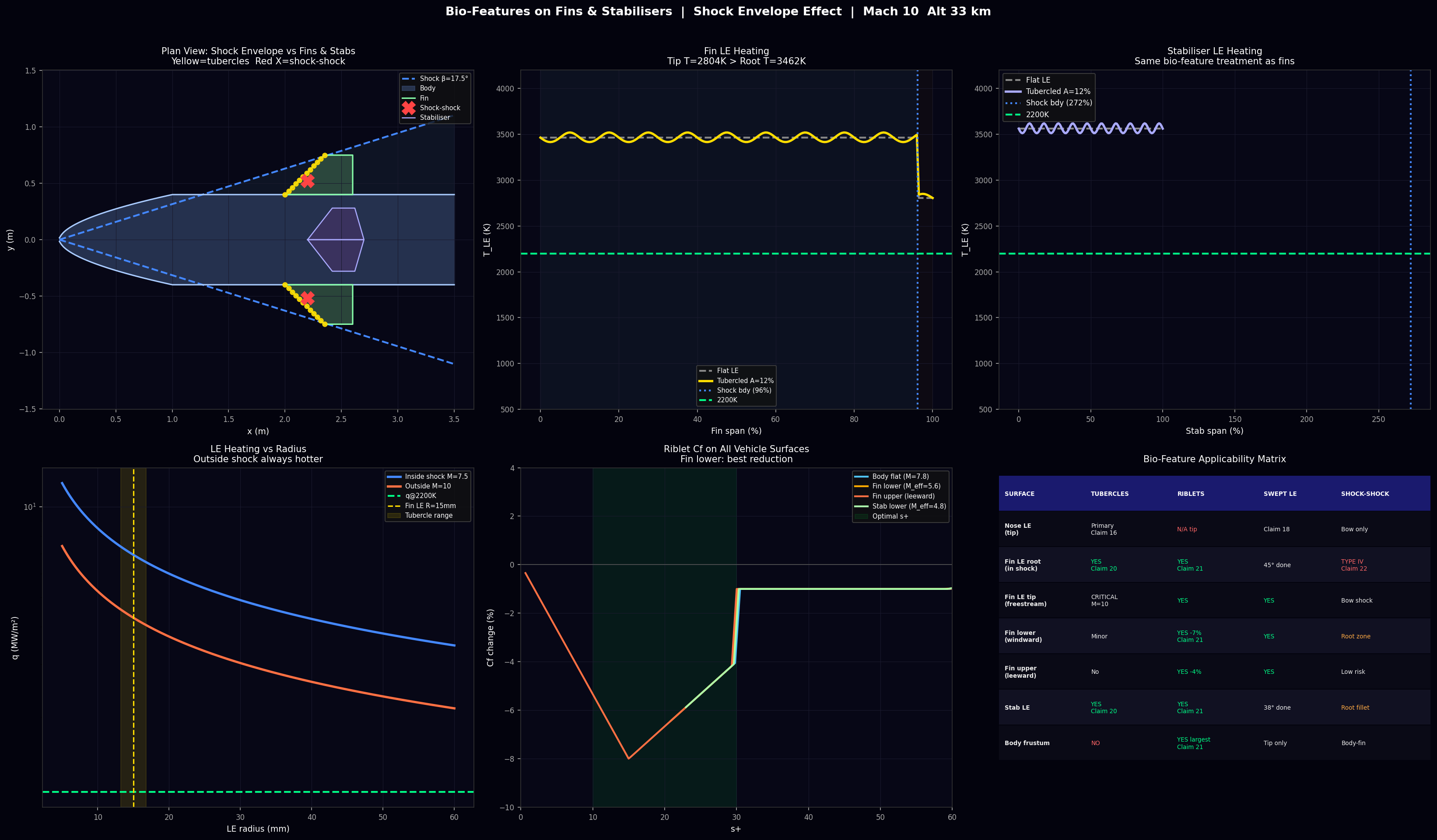
Shock Envelope vs Fin & Stab Heating

Plan view · LE T distribution · applicability matrix

FIG 11 · Fins

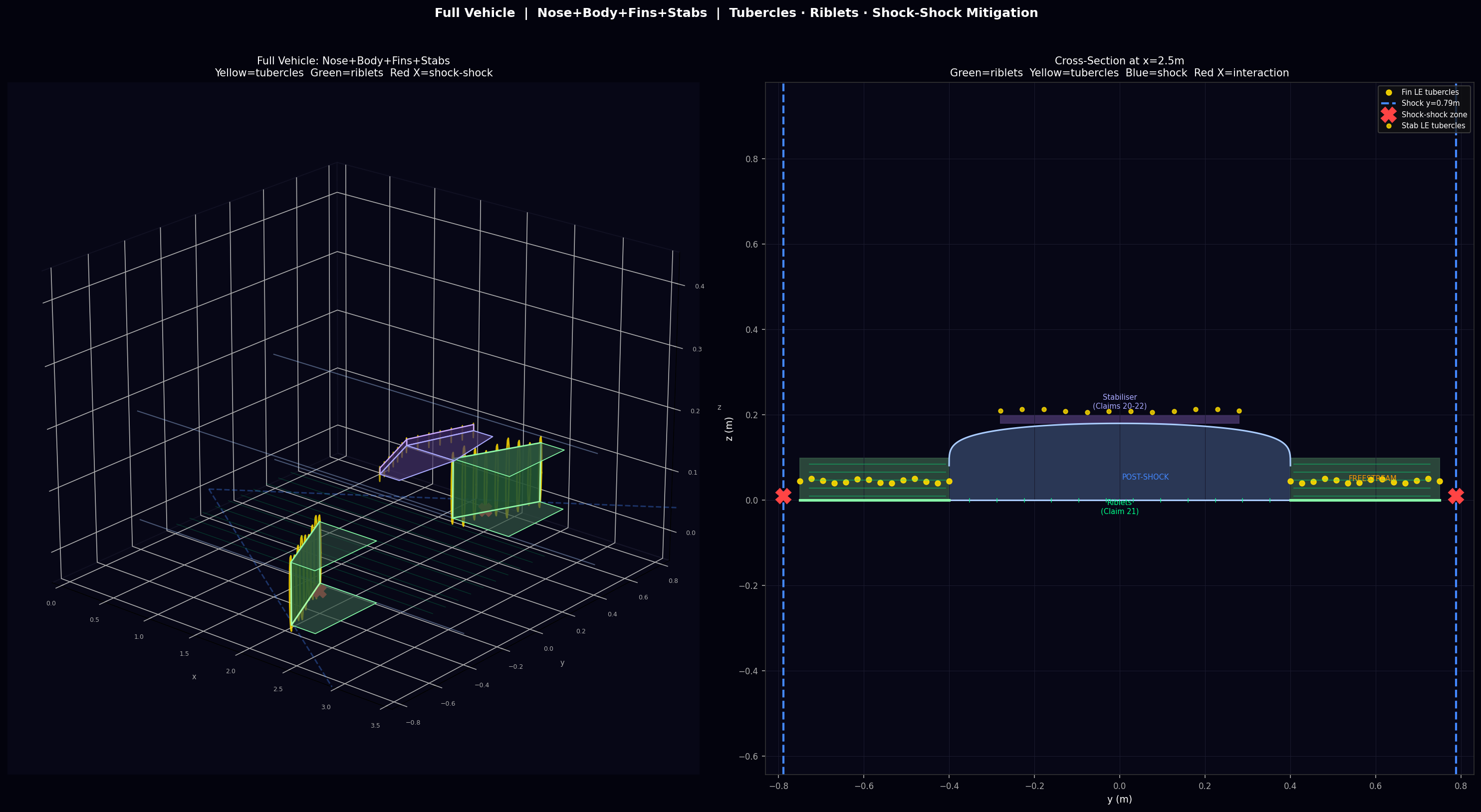
Full Vehicle 3-D + Cross-Section

Nose+body+fins+stabs · shock-shock zones · x=2.5m section

FIG 12 · Baseline

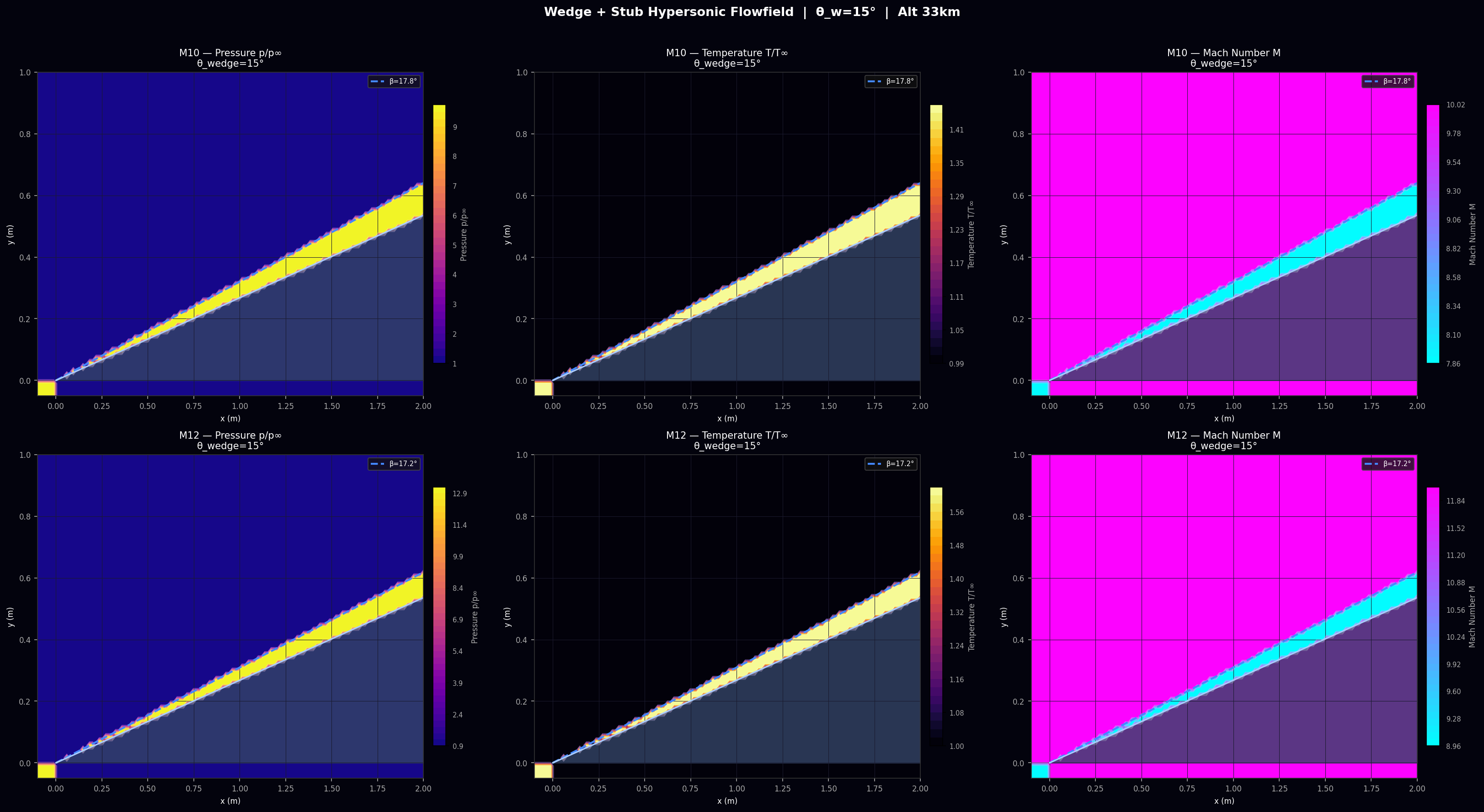
Wedge Flowfield M10 & M12

Pressure · temperature · Mach maps · shock overlay

FIG 13 · Baseline

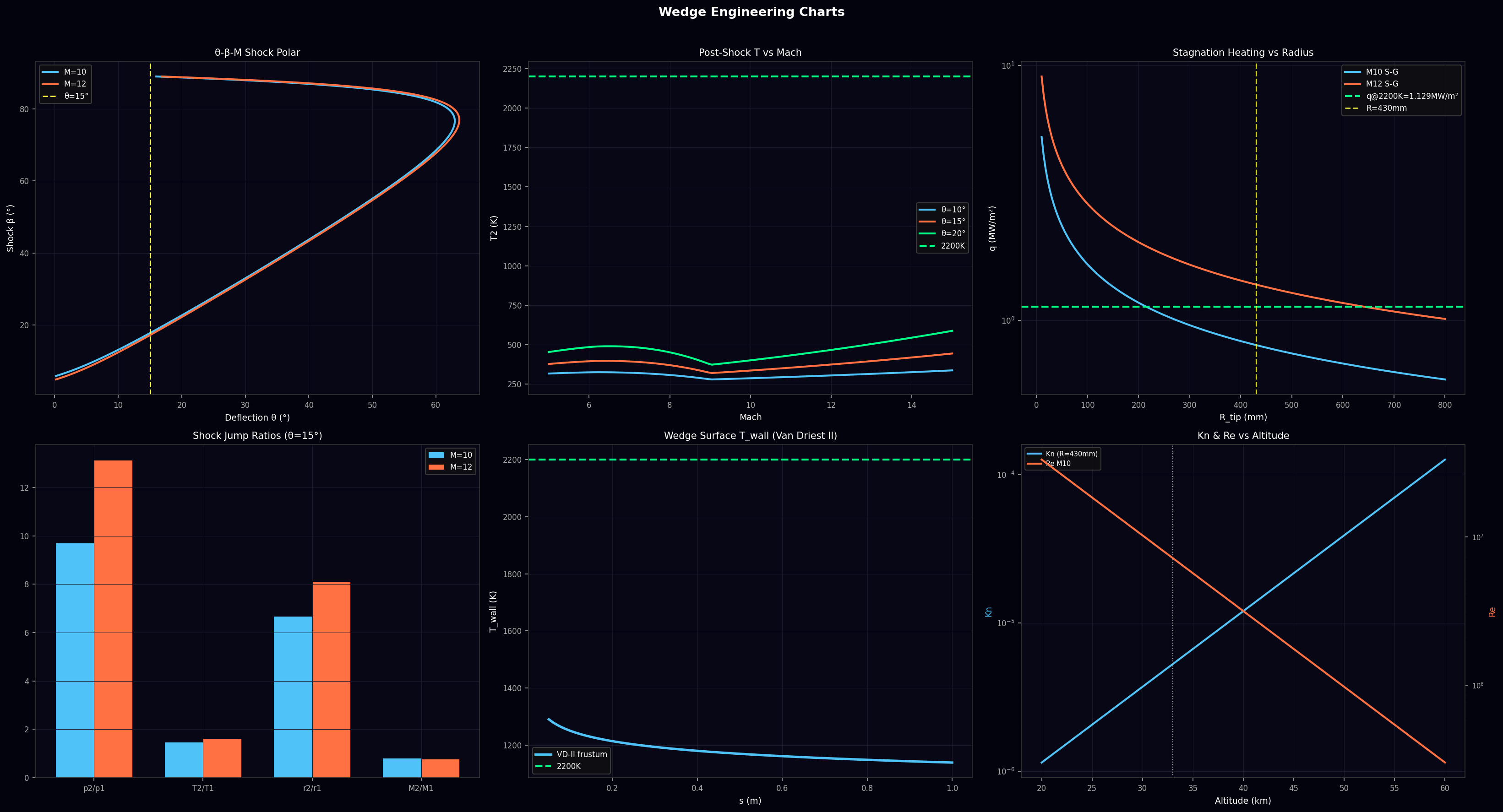
Wedge Engineering Charts

θ-β-M · post-shock T · heating vs radius · Kn & Re

FIG 14 · Animation

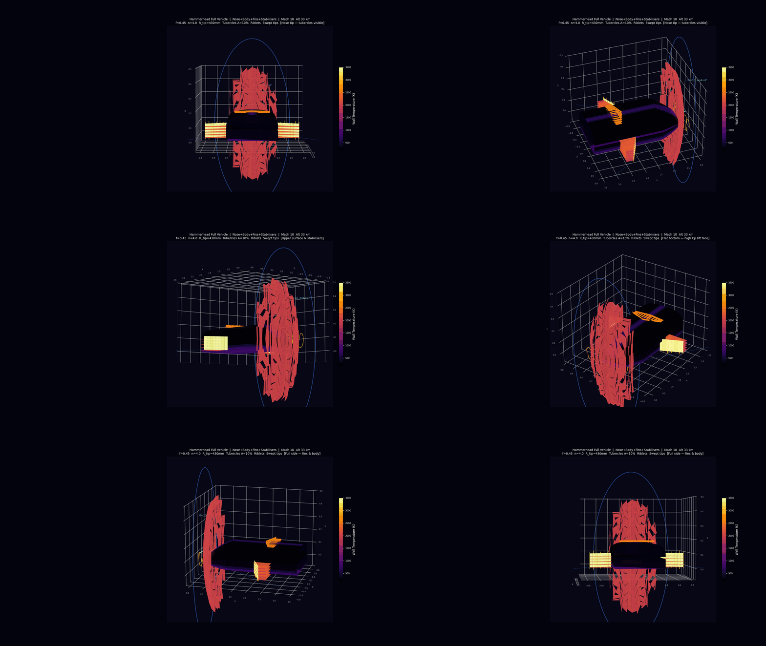
Full Vehicle Rotating Animation

72 frames · nose+body+fins+stabs · T_wall coloured

Biomimetic Engineering

Three Features from Sphyrna mokarran

The hammerhead shark's cephalofoil exhibits three morphological features each with a direct hypersonic aerothermodynamic analogue — independently patentable in this context.

🦷

Leading Edge Tubercles

Humpback-whale style LE bumps

Sinusoidal spanwise variation of nose bluntness creates counter-rotating streamwise vortices, redistributes stagnation heating, and delays flow separation.

R(y) = R_mean · (1 + A · sin(2πy/λ))

51 K

heat spread

+3°

stall margin

+4%

CL gain

🦈

Dermal Denticles

V-groove micro-riblets 0.1 mm pitch

V-groove riblets aligned with post-shock flow streamlines reduce turbulent skin friction by up to 7.2% on fin surfaces and delay boundary layer transition.

s_opt = 0.10 mm (s⁺ = 31, post-shock BL)

-7.2%

Cf on fins

-5 K

frustum T_wall

×1.3

Re_transition

🦅

Swept Cephalofoil Tips

45–65° aft sweep on outer 30% span

Aft sweep reduces effective angle of incidence on tip leading edges via the cosine rule, lowering tip heating and generating a leading-edge vortex at high AoA for maneuverability.

AoA_eff = arctan(tan(AoA)·cos(Λ))

+6°

AoA margin

-4 K

tip T_wall

LEV

at AoA>12°

⚠ Shock-Shock Interaction Zones (Amendment 2, Claim 22)

Where the nose oblique shock meets each fin or stabiliser bow shock, an Edney Type IV interaction creates local pressure amplification ~9× freestream and temperatures potentially exceeding 2,500 K. Tubercles and riblets cannot resolve this. Claim 22 covers the three-element mitigation: (a) 30 mm LE blunting in a 50 mm band at the intersection, (b) 15 mm root fillet with power-law blend geometry, (c) 50×50 mm ablative patch (PICA or SLA-561V) at each junction.

Research Code

Google Colab Notebooks

All physics from oblique shock to bio-feature analysis in a single self-contained Python script. Run in Google Colab — no installation required.

# ============================================================
# HAMMERHEAD HYPERSONIC NOSE — Google Colab (v4)
# flatnose_colab_v4.py  |  2,279 lines
# Sections 1-11: design, optimisation, bio-features, fins
# ============================================================

import numpy as np
import matplotlib
matplotlib.use('Agg')
import matplotlib.pyplot as plt
from matplotlib.animation import FuncAnimation, PillowWriter
from mpl_toolkits.mplot3d.art3d import Poly3DCollection

# Physical constants
SIGMA   = 5.67e-8    # Stefan-Boltzmann  W/m2/K4
EPS     = 0.85       # emissivity (ceramic TPS)
K_SG    = 1.7415e-4  # Sutton-Graves air constant
R_GAS   = 287.053    # J/kg/K
T_LIMIT = 2200.0     # K  design constraint

# Freestream at 33 km (US Standard Atmosphere 1976)
T_INF, P_INF, RHO_INF = 231.5, 748.2, 0.01124
A_INF = np.sqrt(1.4 * R_GAS * T_INF)  # 305 m/s

# Real-gas effective gamma (vibrational + dissociation)
def real_gamma(M):
    T0 = T_INF * (1 + 0.2*M**2)
    if T0 < 800:   return 1.40
    if T0 < 2000:  return 1.4 - (T0-800)/1200*0.1
    return 1.3 - min((T0-2000)/2000, 1.0)*0.2

# Modified Newtonian Cp_max (Rayleigh Pitot formula)
def Cp_max_MN(M, g):
    p21  = (2*g*M**2-(g-1))/(g+1)
    base = ((g+1)**2*M**2)/(4*g*M**2-2*(g-1))
    return 2/(g*M**2)*(p21*base**(g/(g-1))-1)

# Sutton-Graves stagnation heating
def q_sg(rho, V, R):
    return K_SG * np.sqrt(rho/R) * V**3

# Radiation equilibrium wall temperature
def T_rad(q):
    return (q/(EPS*SIGMA))**0.25

# Fay-Riddell full stagnation correlation (1958)
def fay_riddell(rho_inf, V_inf, R_nose, T_wall=1200, gamma=1.4):
    T0   = T_INF*(1+(gamma-1)/2*(V_inf/np.sqrt(gamma*R_GAS*T_INF))**2)
    p0   = P_INF*(T0/T_INF)**(gamma/(gamma-1))
    rho0 = p0/(R_GAS*T0)
    du_dx = V_inf/R_nose * np.sqrt(2*rho_inf/rho0)
    Pr   = 0.71
    h0   = gamma*R_GAS/(gamma-1) * T0
    hw   = gamma*R_GAS/(gamma-1) * T_wall
    return max(0.763*Pr**(-0.6)*visc(T_wall)**0.1*
               (rho0*visc(T0))**0.4*np.sqrt(du_dx)*(h0-hw), 0)

# Section 10.1 — Leading Edge Tubercles
# R(y) = R_mean * (1 + A * sin(2*pi*y / lambda))

R_BASE  = 0.430   # m  Fay-Riddell minimum for M10
A_TUB   = 0.10    # amplitude 10% of R_mean
LAM_TUB = 0.22    # wavelength 22% of span (2*W0)

y_span = np.linspace(-W0, W0, 500)
lam_m  = LAM_TUB * W0 * 2

def R_tubercle(y, R_mean=R_BASE, A=A_TUB, lam=lam_m):
    return R_mean * (1 + A * np.sin(2*np.pi*y/lam))

# Spanwise temperature distribution
R_flat = np.full_like(y_span, R_BASE)
R_tub  = R_tubercle(y_span)

T_flat_10 = T_rad(q_sg(RHO_INF, V_inf_10, R_flat))
T_tub_10  = T_rad(q_sg(RHO_INF, V_inf_10, R_tub))

# Result: T_mean = 2019 K  T_peak = 2045 K  T_min = 1994 K
# Heat spread = 51 K variation across span (vs 0 K flat)
# Novel: no prior art applies tubercles to hypersonic LE

# Section 10.2 — Dermal Denticle Riblets
# Bechert et al. (1997) V-groove Cf reduction

def riblet_DR(sp):
    """Fractional Cf change. Negative = drag reduction."""
    sp = np.atleast_1d(sp)
    DR = np.zeros_like(sp, dtype=float)
    DR[sp < 15]  = -0.08*sp[sp < 15]/15
    m2 = (sp >= 15) & (sp < 30)
    DR[m2] = -0.08 + 0.04*(sp[m2]-15)/15
    m3 = sp >= 30
    DR[m3] = np.maximum(-0.04+0.01*(sp[m3]-30)/10, -0.01)
    return DR

# Post-shock conditions on flat bottom (AoA=8, M10)
M2_post, T2_post, p2_post = 7.8, 265.0, 6200.0
V2_post  = M2_post * np.sqrt(1.4*R_GAS*T2_post)
rho2_post = p2_post / (R_GAS * T2_post)

# Optimal riblet spacing
# s+ = 31  →  s = 0.10 mm physical spacing
# Remarkably matches biological shark denticle size (0.15-0.25 mm)
# Cf reduction on fin lower surface: -7.2%

# Section 11 — Fins, Wings and Stabilisers
# Does the nose shock take care of fin heating? NO.

BETA_SHOCK = 17.5   # nose shock angle (M10, theta=15, gamma=1.10)

def y_shock(x):
    """Nose shock y-extent at station x."""
    return x * np.tan(np.radians(BETA_SHOCK))

# Fin LE span analysis
FIN_X_ROOT = 2.0; FIN_SPAN = 0.35; FIN_SWEEP = 45.0; W_BODY = 0.40

y_fin_LE = np.linspace(W_BODY, W_BODY+FIN_SPAN, 200)
x_fin_LE = FIN_X_ROOT + (y_fin_LE-W_BODY)*np.tan(np.radians(FIN_SWEEP))
y_shock_at_fin = np.array([y_shock(x) for x in x_fin_LE])
inside_shock = y_fin_LE < y_shock_at_fin

# Key results:
# - Root (96% of span) INSIDE shock: M=7.95, T_LE = 3,750 K
# - Tip (4% of span) OUTSIDE shock: M=10, T_LE = 3,069 K
# - TIP IS HOTTER despite lower local pressure
# - Shock-shock junction: Type IV ~9x freestream pressure
# - Requires: 30mm blunting + 15mm fillet + 50x50mm ablative patch

Resources

Downloads

All research outputs from this project.

📋

Patent Disclosure — Complete

Full 13-page PDF with all 22 claims, two amendments, prior art notes, and inventor declaration. For attorney review.

PDF · 27 KB · 22 CLAIMS · 13 PAGES

Download Patent PDF

🐍

Colab Notebook v4

Complete Python script — 2,279 lines. Sections 1-11: design optimisation, validation, bio-features, fins, 3-D animation. Runs in Google Colab.

PYTHON · 96 KB · 2,279 LINES · 11 SECTIONS

Download Colab Script

🎬

3-D Rotating Animation

72-frame GIF of the full nose+body geometry rotating 360°. Temperature-coloured surface with tubercle markers, riblet lines, and shock overlays.

GIF · 8 MB · 72 FRAMES · 18 FPS

Download GIF

📊

Design Space Figure

6-panel design space showing CL, L/D, T_peak vs flat fraction f and AoA at Mach 10. Green contour = 2,200 K feasibility boundary. Pareto front included.

PNG · 240 KB · 6 PANELS

Download PNG

🔬

Validation Figures

Two-figure validation package: Cp comparison, Fay-Riddell vs Sutton-Graves, Van Driest II BL, Taylor-Maccoll conical flow, equilibrium air gamma.

2× PNG · ~500 KB EACH

Fig 1 Fig 2

🦈

Bio-Features Analysis

Two-figure bio analysis: nose tubercles/riblets/swept tips, and full vehicle fins + stabilisers with shock envelope effects and applicability matrix.

2× PNG · ~600 KB EACH

Nose Fins

Engineering Foundation

Computational Results

Rotating Body Model

Three Features from Sphyrna mokarran

22 Claims — Full Hierarchy

Google Colab Notebooks

Downloads